

Feed aggregator
Rownum quiz
Here’s a silly little puzzle that baffled me for a few moments until I spotted my typing error. It starts with a small table I’d created to hold a few rows, and then deletes most of them. Here’s a statement to create and populate the table:
create table t1 (id number , c1 clob)
lob(c1) store as basicfile text_lob (
        retention disable storage in row
);

insert into t1
select  rownum, rpad(rownum,200,'0')
from    all_objects
where   rownum <= 1000
;

commit;
Here’s what I meant to type to delete most of the data – followed by the response from SQL*Plus:
SQL> delete from t1 where mod(id,20) != 0;

950 rows deleted.
Here’s what I actually typed, with the response, that gave me a “What?!” moment:
SQL> delete from t1 where mod(rownum,20) != 0;

19 rows deleted.
I don’t think it will take long for you to work out why the result is so different; but I think it’s a nice warning about what can happen if you get a bit casual about using rownum.
Local RAG Explained with Unstructured and LangChain
Is it a must to run pupbld.sql as system
Mixed version dataguard
How to call rest api which accept x-www-form-urlencoded in PL/SQL procedure in Apex
Error in pl/sql code

Oracle Is Guilty Until Proven Innocent
Received email from Technical Lead | Senior Manager for the following errors.
Error Description: 0: Invalid pool name ‘oraclePool’ while getting a database connection.
Please check for consistency of the properties files or BPML
Time of Event: 20240419141429
Workflow Id: 88867
First inclination is to check Oracle database parameters (sessions and processes) which wasted time on a wild goose chase.
I am by no mean an expert but Google is your friend.
It puzzle me how a Technical Lead | Senior Manager does not know how to Google.
LMGTFY – Let Me Google That For You for all those people who find it more convenient to bother you with their question rather than to Google it for themselves.
How to update a user defined database package in production
Another file system for Linux: bcachefs (2) – multi device file systems
In the last post, we’ve looked at the very basics when it comes to bcachefs, a new file system which was added to the Linux kernel starting from version 6.7. While we’ve already seen how easy it is to create a new file system using a single device, encrypt and/or compress it and that check summing of meta data and user data is enabled by default, there is much more you can do with bcachefs. In this post we’ll look at how you can work with a file system that spans multiple devices, which is quite common in today’s infrastructures.
When we looked at the devices available to the system in the last post, it looked like this:
tumbleweed:~ $ lsblk | grep -w "4G"
└─vda3 254:3    0  1.4G  0 part [SWAP]
vdb    254:16   0    4G  0 disk
vdc    254:32   0    4G  0 disk
vdd    254:48   0    4G  0 disk
vde    254:64   0    4G  0 disk
vdf    254:80   0    4G  0 disk
vdg    254:96   0    4G  0 disk
This means we have six unused block devices to play with. Lets start again with the most simple case, one device, one file system:
tumbleweed:~ $ bcachefs format --force /dev/vdb
tumbleweed:~ $ mount /dev/vdb /mnt/dummy/
tumbleweed:~ $ df -h | grep dummy
/dev/vdb        3.7G  2.0M  3.6G   1% /mnt/dummy
Assuming we’re running out of space on that file system and we want to add another device, how does work?
tumbleweed:~ $ bcachefs device add /mnt/dummy/ /dev/vdc
tumbleweed:~ $ df -h | grep dummy
/dev/vdb:/dev/vdc  7.3G  2.0M  7.2G   1% /mnt/dummy
Quite easy, and no separate step required to extend the file system, this was done automatically which is quite nice. You can even go a step further and specify how large the file system should be on the new device (which doesn’t make much sense in this case):
tumbleweed:~ $ bcachefs device add --fs_size=4G /mnt/dummy/ /dev/vdd
tumbleweed:~ $ df -h | grep mnt
/dev/vdb:/dev/vdc:/dev/vdd   11G  2.0M   11G   1% /mnt/dummy
Let’s remove this configuration and then create a file system with multiple devices right from the beginning:
tumbleweed:~ $ bcachefs format --force /dev/vdb /dev/vdc
Now we formatted two devices at once, which is great, but how can we mount that? This will obviously not work:
tumbleweed:~ $ mount /dev/vdb /dev/vdc /mnt/dummy/
mount: bad usage
Try 'mount --help' for more information.
The syntax is a bit different, so either do it it with “mount”:
tumbleweed:~ $ mount -t bcachefs /dev/vdb:/dev/vdc /mnt/dummy/
tumbleweed:~ $ df -h | grep dummy
/dev/vdb:/dev/vdc  7.3G  2.0M  7.2G   1% /mnt/dummy
… or use the “bcachefs” utility using the same syntax for the list of devices:
tumbleweed:~ $ umount /mnt/dummy
tumbleweed:~ $ bcachefs mount /dev/vdb:/dev/vdc /mnt/dummy/
tumbleweed:~ $ df -h | grep dummy
/dev/vdb:/dev/vdc  7.3G  2.0M  7.2G   1% /mnt/dummy
What is a bit annoying is, that you need to know which devices you can still add, as you won’t see this in the “lsblk” output”:
tumbleweed:~ $ lsblk | grep -w "4G"
└─vda3 254:3    0  1.4G  0 part [SWAP]
vdb    254:16   0    4G  0 disk /mnt/dummy
vdc    254:32   0    4G  0 disk
vdd    254:48   0    4G  0 disk
vde    254:64   0    4G  0 disk
vdf    254:80   0    4G  0 disk
vdg    254:96   0    4G  0 disk
You do see it, however in the “df -h” output:
tumbleweed:~ $ df -h | grep dummy
/dev/vdb:/dev/vdc  7.3G  2.0M  7.2G   1% /mnt/dummy
Another way to get those details is once more to use the “bcachefs” utility:
tumbleweed:~ $ bcachefs fs usage /mnt/dummy/
Filesystem: d6f85f8f-dc12-4e83-8547-6fa8312c8eca
Size:                     7902739968
Used:                       76021760
Online reserved:                   0

Data type       Required/total  Durability    Devices
btree:          1/1             1             [vdb]                1048576
btree:          1/1             1             [vdc]                1048576

(no label) (device 0):           vdb              rw
                                data         buckets    fragmented
  free:                   4256956416           16239
  sb:                        3149824              13        258048
  journal:                  33554432             128
  btree:                     1048576               4
  user:                            0               0
  cached:                          0               0
  parity:                          0               0
  stripe:                          0               0
  need_gc_gens:                    0               0
  need_discard:                    0               0
  capacity:               4294967296           16384

(no label) (device 1):           vdc              rw
                                data         buckets    fragmented
  free:                   4256956416           16239
  sb:                        3149824              13        258048
  journal:                  33554432             128
  btree:                     1048576               4
  user:                            0               0
  cached:                          0               0
  parity:                          0               0
  stripe:                          0               0
  need_gc_gens:                    0               0
  need_discard:                    0               0
  capacity:               4294967296           16384
Note that shrinking a file system on a device is currently not supported, only growing.
In the next post we’ll look at how you can mirror your data across multiple devices.
L’article Another file system for Linux: bcachefs (2) – multi device file systems est apparu en premier sur dbi Blog.
How to Quantize a Model with Hugging Face Quanto
This video is a hands-on step-by-step primer about how to quantize any model using Hugging Face Quanto which is a versatile pytorch quantization toolkit.
!pip install transformers==4.35.0
!pip install quanto==0.0.11
!pip install torch==2.1.1
!pip install sentencepiece==0.2.0
model_name = "google/flan-t5-small"
import sentencepiece as spm
from transformers import T5Tokenizer, T5ForConditionalGeneration
tokenizer = T5Tokenizer.from_pretrained("google/flan-t5-small")
model = T5ForConditionalGeneration.from_pretrained("google/flan-t5-small")
input_text = "Meaning of happiness is "
input_ids = tokenizer(input_text, return_tensors="pt").input_ids
outputs = model.generate(input_ids)
print(tokenizer.decode(outputs[0]))
from helper import compute_module_sizes
module_sizes = compute_module_sizes(model)
print(f"The model size is {module_sizes[''] * 1e-9} GB")
from quanto import quantize, freeze
import torch
quantize(model, weights=torch.int8, activations=None)
freeze(model)
module_sizes = compute_module_sizes(model)
print(f"The model size is {module_sizes[''] * 1e-9} GB")
input_text = "Meaning of happiness is "
input_ids = tokenizer(input_text, return_tensors="pt").input_ids
outputs = model.generate(input_ids)
print(tokenizer.decode(outputs[0]))
How to do RAG in OpenAI GPT4 Locally with File Search
This video is a hands-on step-by-step primer about how to use RAG with Open AI File Search. OpenAI now supports RAG which means that now you can attach your own files and custom data to OpenAI assistant and talk to your documents with GPT4.
Make sure you have installed latest version of openai on your local system:
pip install openai --upgrade
also make sure to have data.txt in the same folder as your script.
How to Use LLM Function Calling Locally for Free
Function calling in AI simply means that you can call external APIs from within your AI-powered application. Whenever you read that a model can do function calling, it means that it can take a natural language query of user and convert it to a function call. Then you can execute that function call to your API endpoint to get the data, and give it to LLM as additional context and get more grounded latest response as per your application requirement.
Another file system for Linux: bcachefs (1) – basics
When Linux 6.7 (already end of life) was released some time ago another file system made it into the kernel: bcachefs. This is another copy on write file system like ZFS or Btrfs. The goal of this post is not to compare those in regards to features and performance, but just to give you the necessary bits to get started with it. If you want to try this out for yourself, you obviously need at least version 6.7 of the Linux kernel. You can either build it yourself or you can use the distribution of your choice which ships at least with kernel 6.7 as an option. I’ll be using openSUSE Tumbleweed as this is a rolling release and new kernel versions make it into the distribution quite fast after they’ve been released.
When you install Tumbleweed as of today, you’ll get a 6.8 kernel which is fine if you want to play around with bcachefs:
tumbleweed:~ $ uname -a
Linux tumbleweed 6.8.5-1-default #1 SMP PREEMPT_DYNAMIC Thu Apr 11 04:31:19 UTC 2024 (542f698) x86_64 x86_64 x86_64 GNU/Linux
Let’s start very simple: Once device, on file system. Usually you create a new file system with the mkfs command, but you’ll quickly notice that there is nothing for bcachefs:
tumbleweed:~ $ mkfs.[TAB][TAB]
mkfs.bfs     mkfs.btrfs   mkfs.cramfs  mkfs.ext2    mkfs.ext3    mkfs.ext4    mkfs.fat     mkfs.minix   mkfs.msdos   mkfs.ntfs    mkfs.vfat
By default there is also no command which starts with “bca”:
tumbleweed:~ # bca[TAB][TAB]
The utilities you need to get started need to be installed on Tumbleweed:
tumbleweed:~ $ zypper se bcachefs
Loading repository data...
Reading installed packages...

S | Name           | Summary                              | Type
--+----------------+--------------------------------------+--------
  | bcachefs-tools | Configuration utilities for bcachefs | package

tumbleweed:~ $ zypper in -y bcachefs-tools
Loading repository data...
Reading installed packages...
Resolving package dependencies...

The following 2 NEW packages are going to be installed:
  bcachefs-tools libsodium23

2 new packages to install.
Overall download size: 1.4 MiB. Already cached: 0 B. After the operation, additional 3.6 MiB will be used.

Backend:  classic_rpmtrans
Continue? [y/n/v/...? shows all options] (y): y
Retrieving: libsodium23-1.0.18-2.16.x86_64 (Main Repository (OSS))                                                                                        (1/2), 169.7 KiB
Retrieving: libsodium23-1.0.18-2.16.x86_64.rpm ...........................................................................................................[done (173.6 KiB/s)]
Retrieving: bcachefs-tools-1.6.4-1.2.x86_64 (Main Repository (OSS))                                                                                       (2/2),   1.2 MiB
Retrieving: bcachefs-tools-1.6.4-1.2.x86_64.rpm ............................................................................................................[done (5.4 MiB/s)]

Checking for file conflicts: ...........................................................................................................................................[done]
(1/2) Installing: libsodium23-1.0.18-2.16.x86_64 .......................................................................................................................[done]
(2/2) Installing: bcachefs-tools-1.6.4-1.2.x86_64 ......................................................................................................................[done]
Running post-transaction scripts .......................................................................................................................................[done]
This will give you “mkfs.bcachefs” and all the other utilities you’ll need to play with it.
I’ve prepared six small devices I can play with:
tumbleweed:~ $ lsblk
NAME   MAJ:MIN RM  SIZE RO TYPE MOUNTPOINTS
sr0     11:0    1  276M  0 rom
vda    254:0    0   20G  0 disk
├─vda1 254:1    0    8M  0 part
├─vda2 254:2    0 18.6G  0 part /var
│                               /srv
│                               /usr/local
│                               /opt
│                               /root
│                               /home
│                               /boot/grub2/x86_64-efi
│                               /boot/grub2/i386-pc
│                               /.snapshots
│                               /
└─vda3 254:3    0  1.4G  0 part [SWAP]
vdb    254:16   0    4G  0 disk
vdc    254:32   0    4G  0 disk
vdd    254:48   0    4G  0 disk
vde    254:64   0    4G  0 disk
vdf    254:80   0    4G  0 disk
vdg    254:96   0    4G  0 disk
In the most simple form (one device, one file system) you might start like this:
tumbleweed:~ $ bcachefs format /dev/vdb
External UUID:                              127933ff-575b-484f-9eab-d0bf5dbf52b2
Internal UUID:                              fbf59149-3dc4-4871-bfb5-8fb910d0529f
Magic number:                               c68573f6-66ce-90a9-d96a-60cf803df7ef
Device index:                               0
Label:
Version:                                    1.6: btree_subvolume_children
Version upgrade complete:                   0.0: (unknown version)
Oldest version on disk:                     1.6: btree_subvolume_children
Created:                                    Wed Apr 17 10:39:58 2024
Sequence number:                            0
Time of last write:                         Thu Jan  1 01:00:00 1970
Superblock size:                            960 B/1.00 MiB
Clean:                                      0
Devices:                                    1
Sections:                                   members_v1,members_v2
Features:                                   new_siphash,new_extent_overwrite,btree_ptr_v2,extents_above_btree_updates,btree_updates_journalled,new_varint,journal_no_flush,alloc_v2,extents_across_btree_nodes
Compat features:

Options:
  block_size:                               512 B
  btree_node_size:                          256 KiB
  errors:                                   continue [ro] panic
  metadata_replicas:                        1
  data_replicas:                            1
  metadata_replicas_required:               1
  data_replicas_required:                   1
  encoded_extent_max:                       64.0 KiB
  metadata_checksum:                        none [crc32c] crc64 xxhash
  data_checksum:                            none [crc32c] crc64 xxhash
  compression:                              none
  background_compression:                   none
  str_hash:                                 crc32c crc64 [siphash]
  metadata_target:                          none
  foreground_target:                        none
  background_target:                        none
  promote_target:                           none
  erasure_code:                             0
  inodes_32bit:                             1
  shard_inode_numbers:                      1
  inodes_use_key_cache:                     1
  gc_reserve_percent:                       8
  gc_reserve_bytes:                         0 B
  root_reserve_percent:                     0
  wide_macs:                                0
  acl:                                      1
  usrquota:                                 0
  grpquota:                                 0
  prjquota:                                 0
  journal_flush_delay:                      1000
  journal_flush_disabled:                   0
  journal_reclaim_delay:                    100
  journal_transaction_names:                1
  version_upgrade:                          [compatible] incompatible none
  nocow:                                    0

members_v2 (size 144):
Device:                                     0
  Label:                                    (none)
  UUID:                                     bb28c803-621a-4007-af13-a9218808de8f
  Size:                                     4.00 GiB
  read errors:                              0
  write errors:                             0
  checksum errors:                          0
  seqread iops:                             0
  seqwrite iops:                            0
  randread iops:                            0
  randwrite iops:                           0
  Bucket size:                              256 KiB
  First bucket:                             0
  Buckets:                                  16384
  Last mount:                               (never)
  Last superblock write:                    0
  State:                                    rw
  Data allowed:                             journal,btree,user
  Has data:                                 (none)
  Durability:                               1
  Discard:                                  0
  Freespace initialized:                    0
mounting version 1.6: btree_subvolume_children
initializing new filesystem
going read-write
initializing freespace
This is already ready to mount and we have our first bcachfs file system:
tumbleweed:~ $ mkdir /mnt/dummy
tumbleweed:~ $ mount /dev/vdb /mnt/dummy
tumbleweed:~ $ df -h | grep dummy
/dev/vdb        3.7G  2.0M  3.6G   1% /mnt/dummy
If you need encryption, this is supported as well and obviously is asking you for a passphrase when you format the device:
tumbleweed:~ $ umount /mnt/dummy
tumbleweed:~ $ bcachefs format --encrypted --force /dev/vdb
Enter passphrase:
Enter same passphrase again:
/dev/vdb contains a bcachefs filesystem
External UUID:                              aa0a4742-46ed-4228-a590-62b8e2de7633
Internal UUID:                              800b2306-3900-47fb-9a42-2f7e75baec99
Magic number:                               c68573f6-66ce-90a9-d96a-60cf803df7ef
Device index:                               0
Label:
Version:                                    1.4: member_seq
Version upgrade complete:                   0.0: (unknown version)
Oldest version on disk:                     1.4: member_seq
Created:                                    Wed Apr 17 10:46:06 2024
Sequence number:                            0
Time of last write:                         Thu Jan  1 01:00:00 1970
Superblock size:                            1.00 KiB/1.00 MiB
Clean:                                      0
Devices:                                    1
Sections:                                   members_v1,crypt,members_v2
Features:
Compat features:

Options:
  block_size:                               512 B
  btree_node_size:                          256 KiB
  errors:                                   continue [ro] panic
  metadata_replicas:                        1
  data_replicas:                            1
  metadata_replicas_required:               1
  data_replicas_required:                   1
  encoded_extent_max:                       64.0 KiB
  metadata_checksum:                        none [crc32c] crc64 xxhash
  data_checksum:                            none [crc32c] crc64 xxhash
  compression:                              none
  background_compression:                   none
  str_hash:                                 crc32c crc64 [siphash]
  metadata_target:                          none
  foreground_target:                        none
  background_target:                        none
  promote_target:                           none
  erasure_code:                             0
  inodes_32bit:                             1
  shard_inode_numbers:                      1
  inodes_use_key_cache:                     1
  gc_reserve_percent:                       8
  gc_reserve_bytes:                         0 B
  root_reserve_percent:                     0
  wide_macs:                                0
  acl:                                      1
  usrquota:                                 0
  grpquota:                                 0
  prjquota:                                 0
  journal_flush_delay:                      1000
  journal_flush_disabled:                   0
  journal_reclaim_delay:                    100
  journal_transaction_names:                1
  version_upgrade:                          [compatible] incompatible none
  nocow:                                    0

members_v2 (size 144):
Device:                                     0
  Label:                                    (none)
  UUID:                                     60de61d2-391b-4605-b0da-5f593b7c703f
  Size:                                     4.00 GiB
  read errors:                              0
  write errors:                             0
  checksum errors:                          0
  seqread iops:                             0
  seqwrite iops:                            0
  randread iops:                            0
  randwrite iops:                           0
  Bucket size:                              256 KiB
  First bucket:                             0
  Buckets:                                  16384
  Last mount:                               (never)
  Last superblock write:                    0
  State:                                    rw
  Data allowed:                             journal,btree,user
  Has data:                                 (none)
  Durability:                               1
  Discard:                                  0
  Freespace initialized:                    0
To mount this you’ll need to specify the passphrase given above or it will fail:
tumbleweed:~ $ mount /dev/vdb /mnt/dummy/
Enter passphrase:
ERROR - bcachefs::commands::cmd_mount: Fatal error: failed to verify the password
tumbleweed:~ $ mount /dev/vdb /mnt/dummy/
Enter passphrase:
tumbleweed:~ $ df -h | grep dummy
/dev/vdb        3.7G  2.0M  3.6G   1% /mnt/dummy
tumbleweed:~ $ umount /mnt/dummy
Beside encryption you may also use compression (supported are gzip, lz4 and zstd), e.g.:
tumbleweed:~ $ bcachefs format --compression=lz4 --force /dev/vdb
/dev/vdb contains a bcachefs filesystem
External UUID:                              1ebcfe14-7d6a-43b1-8d48-47bcef0e7021
Internal UUID:                              5117240c-95f1-4c2a-bed4-afb4c4fbb83c
Magic number:                               c68573f6-66ce-90a9-d96a-60cf803df7ef
Device index:                               0
Label:
Version:                                    1.4: member_seq
Version upgrade complete:                   0.0: (unknown version)
Oldest version on disk:                     1.4: member_seq
Created:                                    Wed Apr 17 10:54:02 2024
Sequence number:                            0
Time of last write:                         Thu Jan  1 01:00:00 1970
Superblock size:                            960 B/1.00 MiB
Clean:                                      0
Devices:                                    1
Sections:                                   members_v1,members_v2
Features:
Compat features:

Options:
  block_size:                               512 B
  btree_node_size:                          256 KiB
  errors:                                   continue [ro] panic
  metadata_replicas:                        1
  data_replicas:                            1
  metadata_replicas_required:               1
  data_replicas_required:                   1
  encoded_extent_max:                       64.0 KiB
  metadata_checksum:                        none [crc32c] crc64 xxhash
  data_checksum:                            none [crc32c] crc64 xxhash
  compression:                              lz4
  background_compression:                   none
  str_hash:                                 crc32c crc64 [siphash]
  metadata_target:                          none
  foreground_target:                        none
  background_target:                        none
  promote_target:                           none
  erasure_code:                             0
  inodes_32bit:                             1
  shard_inode_numbers:                      1
  inodes_use_key_cache:                     1
  gc_reserve_percent:                       8
  gc_reserve_bytes:                         0 B
  root_reserve_percent:                     0
  wide_macs:                                0
  acl:                                      1
  usrquota:                                 0
  grpquota:                                 0
  prjquota:                                 0
  journal_flush_delay:                      1000
  journal_flush_disabled:                   0
  journal_reclaim_delay:                    100
  journal_transaction_names:                1
  version_upgrade:                          [compatible] incompatible none
  nocow:                                    0

members_v2 (size 144):
Device:                                     0
  Label:                                    (none)
  UUID:                                     3bae44f0-3cd4-4418-8556-4342e74c22d1
  Size:                                     4.00 GiB
  read errors:                              0
  write errors:                             0
  checksum errors:                          0
  seqread iops:                             0
  seqwrite iops:                            0
  randread iops:                            0
  randwrite iops:                           0
  Bucket size:                              256 KiB
  First bucket:                             0
  Buckets:                                  16384
  Last mount:                               (never)
  Last superblock write:                    0
  State:                                    rw
  Data allowed:                             journal,btree,user
  Has data:                                 (none)
  Durability:                               1
  Discard:                                  0
  Freespace initialized:                    0
tumbleweed:~ $ mount /dev/vdb /mnt/dummy/
tumbleweed:~ $ df -h | grep dummy
/dev/vdb        3.7G  2.0M  3.6G   1% /mnt/dummy
Meta data and data check sums are enabled by default:
tumbleweed:~ $ bcachefs show-super -l /dev/vdb | grep -i check
  metadata_checksum:                        none [crc32c] crc64 xxhash
  data_checksum:                            none [crc32c] crc64 xxhash
  checksum errors:                          0
That’s it for the very basics. In the next post we’ll look at multi device file systems.
L’article Another file system for Linux: bcachefs (1) – basics est apparu en premier sur dbi Blog.
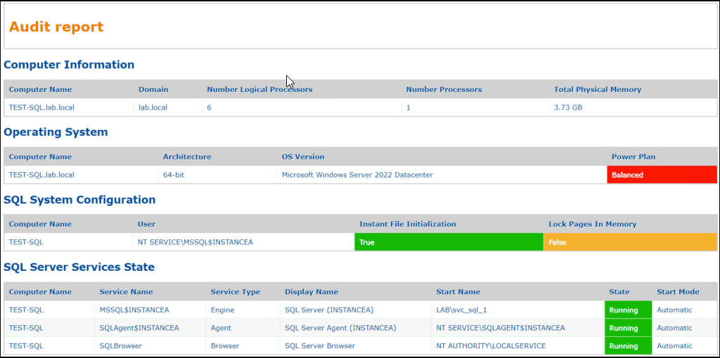
Build SQL Server audit reports with Powershell
When you are tasked with conducting an audit at a client’s site or on the environment you manage, you might find it necessary to automate the audit process in order to save time. However, it can be challenging to extract information from either the PowerShell console or a text file.
Here, the idea would be to propose a solution that could generate audit reports to quickly identify how the audited environment is configured. We will attempt to propose a solution that will automate the generation of audit reports.
In broad terms, here are what we will implement:
- Define the environment we wish to audit. We centralize the configuration of our environments and all the parameters we will use.
- Define the checks or tests we would like to perform.
- Execute these checks. In our case, we will mostly use dbatools to perform the checks. However, it’s possible that you may not be able to use dbatools in your environment for security reasons, for example. In that case, you could replace calls to dbatools with calls to PowerShell functions.
- Produce an audit report.
Here are the technologies we will use in our project :
- SQL Server
- Powershell
- Windows Server
- XML, XSLT and JSON
In our example, we use the dbatools module in oder to get some information related to the environment(s) we audit.
Reference : https://dbatools.io/
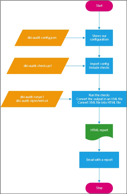
Global architectureHere is how our solution will work :
- We store the configuration of our environment in a JSON file. This avoids storing certain parameters in the PowerShell code.
- We import our configuration (our JSON file). We centralize in one file all the checks, tests to be performed. The configuration stored in the JSON file is passed to the tests.
- We execute all the tests to be performed, then we generate an HTML file (applying an XSLT style sheet) from the collected information.
- We can then send this information by email (for example).
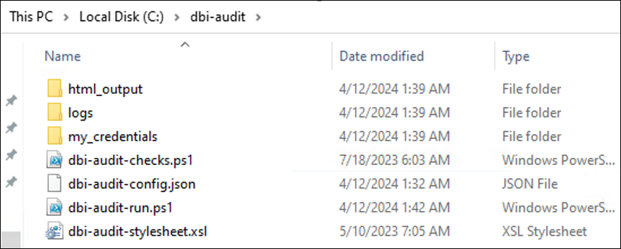
Here are some details about the structure of our project :
FolderTypeFileDescriptionDetailsdbi-auditPS1 filedbi-audit-config.jsonContains some pieces of information related to the environment you would like to audit.The file is called by the dbi-audit-checks.ps1. We import that file and parse it. E.g. if you need to add new servers to audit you can edit that file and run a new audit.dbi-auditPS1 filedbi-audit-checks.ps1Store the checks to perform on the environment(s).That file acts as a “library”, it contains all the checks to perform. It centralizes all the functions.dbi-auditPS1 filedbi-audit-run.ps1Run the checks to perform Transform the output in an html file.It’s the most import file :It runs the checks to perform.
It builds the html report and apply a stylesheet
It can also send by email the related reportdbi-auditXSL filedbi-audit-stylesheet.xslContains the stylesheet to apply to the HTML report.It’s where you will define what you HTML report will look like.html_outputFolder–Will contain the report audit produced.It stores HTML reports.
What does it look like ?
How does it work ?
 Implementation
Code – A basic implementation :
dbi-audit-config.json :
[
	{
		"Name": "dbi-app.computername",
		"Value": [
					  "TEST-SQL"
				  ],
		"Description": "Windows servers list to audit"
	},
	{
		"Name": "dbi-app.sqlinstance",
		"Value": [
					  "TEST-SQL\\INSTANCEA"
				  ],
		"Description": "SQL Server list to audit"
	},
	{
		"Name": "dbi-app.checkcomputersinformation.enabled",
		"Value": "True",
		"Description": "Get some information on OS level"
	},
	{
		"Name": "dbi-app.checkoperatingsystem.enabled",
		"Value": "True",
		"Description": "Perform some OS checks"
	},
	{
		"Name": "dbi-app.checksqlsystemconfiguration.enabled",
		"Value": "True",
		"Description": "Check some SQL Server system settings"
	}
]
dbi-audit-checks.ps1 :
#We import our configuration
$AuditConfig = [PSCustomObject](Get-Content .\dbi-audit-config.json | Out-String | ConvertFrom-Json)

#We retrieve the values contained in our json file. Each value is stored in a variable
$Computers = $AuditConfig | Where-Object { $_.Name -eq 'dbi-app.computername' } | Select-Object Value
$SQLInstances = $AuditConfig | Where-Object { $_.Name -eq 'dbi-app.sqlinstance' } | Select-Object Value
$UnitFileSize = ($AuditConfig | Where-Object { $_.Name -eq 'app.unitfilesize' } | Select-Object Value).Value

#Our configuration file allow to enable or disable some checks. We also retrieve those values.
$EnableCheckComputersInformation = ($AuditConfig | Where-Object { $_.Name -eq 'dbi-app.checkcomputersinformation.enabled' } | Select-Object Value).Value
$EnableCheckOperatingSystem = ($AuditConfig | Where-Object { $_.Name -eq 'dbi-app.checkoperatingsystem.enabled' } | Select-Object Value).Value
$EnableCheckSQLSystemConfiguration = ($AuditConfig | Where-Object { $_.Name -eq 'dbi-app.checksqlsystemconfiguration.enabled' } | Select-Object Value).Value

#Used to invoke command queries
$ComputersList = @()
$ComputersList += $Computers | Foreach-Object {
   $_.Value
}


<#
    Get Computer Information
#>

function CheckComputersInformation()
{
    if ($EnableCheckComputersInformation)
    {
        $ComputersInformationList = @()
        $ComputersInformationList += $Computers | Foreach-Object {
                                                    Get-DbaComputerSystem -ComputerName $_.Value |
                                                        Select-Object ComputerName, Domain, NumberLogicalProcessors,
                                                        NumberProcessors, TotalPhysicalMemory
        }
    }

    return $ComputersInformationList
}


<#
    Get OS Information
#>

function CheckOperatingSystem()
{
    if ($EnableCheckOperatingSystem)
    {
        $OperatingSystemList = @()
        $OperatingSystemList += $Computers | Foreach-Object {
                                                Get-DbaOperatingSystem -ComputerName $_.Value |
                                                    Select-Object ComputerName, Architecture, OSVersion, ActivePowerPlan
        }
    }

    return $OperatingSystemList
}


<#
    Get SQL Server/OS Configuration : IFI, LockPagesInMemory
#>

function CheckSQLSystemConfiguration()
{
    if ($EnableCheckSQLSystemConfiguration)
    {
        $SQLSystemConfigurationList = @()

        $SQLSystemConfigurationList += $Computers | Foreach-Object {
                                                        $ComputerName = $_.Value
                                                        Get-DbaPrivilege -ComputerName $ComputerName |
                                                            Where-Object { $_.User -like '*MSSQL*' } |
                                                                Select-Object ComputerName, User, InstantFileInitialization, LockPagesInMemory
                                                        $ComputerName = $Null
        }
    }

    return $SQLSystemConfigurationList
}
dbi-audit-run.ps1 :
#Our configuration file will accept a parameter. It's the stylesheet to apply to our HTML report
Param(
  [parameter(mandatory=$true)][string]$XSLStyleSheet
)

# We import the checks to run
. .\dbi-audit-checks.ps1


#Setup the XML configuration
$ScriptLocation = Get-Location
$XslOutputPath = "$($ScriptLocation.Path)\$($XSLStyleSheet)"
$FileSavePath = "$($ScriptLocation.Path)\html_output"
[System.XML.XMLDocument]$XmlOutput = New-Object System.XML.XMLDocument
[System.XML.XMLElement]$XmlRoot = $XmlOutput.CreateElement("DbiAuditReport")
$Null = $XmlOutput.appendChild($XmlRoot)

#We run the checks. Instead of manually call all the checks, we store them in array
#We browse that array and we execute the related function
#Each function result is used and append to the XML structure we build
$FunctionsName = @("CheckComputersInformation", "CheckOperatingSystem", "CheckSQLSystemConfiguration")

$FunctionsStore = [ordered] @{}
$FunctionsStore['ComputersInformation'] = CheckComputersInformation
$FunctionsStore['OperatingSystem'] = CheckOperatingSystem
$FunctionsStore['SQLSystemConfiguration'] = CheckSQLSystemConfiguration

$i = 0
$FunctionsStore.Keys | ForEach-Object {

    [System.XML.XMLElement]$xmlSQLChecks = $XmlRoot.appendChild($XmlOutput.CreateElement($FunctionsName[$i]))
    $Results = $FunctionsStore[$_]

    foreach ($Data in $Results)
    {
        $xmlServicesEntry = $xmlSQLChecks.appendChild($XmlOutput.CreateElement($_))

        foreach ($DataProperties in $Data.PSObject.Properties)
        {
            $xmlServicesEntry.SetAttribute($DataProperties.Name, $DataProperties.Value)
        }
    }

    $i++
}

#We create our XML file
$XmlRoot.SetAttribute("EndTime", (Get-Date -Format yyyy-MM-dd_h-mm))
$ReportXMLFileName = [string]::Format("{0}\{1}_DbiAuditReport.xml", $FileSavePath, (Get-Date).tostring("MM-dd-yyyy_HH-mm-ss"))
$ReportHTMLFileName = [string]::Format("{0}\{1}_DbiAuditReport.html", $FileSavePath, (Get-Date).tostring("MM-dd-yyyy_HH-mm-ss"))
$XmlOutput.Save($ReportXMLFileName)

#We apply our XSLT stylesheet
[System.Xml.Xsl.XslCompiledTransform]$XSLT = New-Object System.Xml.Xsl.XslCompiledTransform
$XSLT.Load($XslOutputPath)

#We build our HTML file
$XSLT.Transform($ReportXMLFileName, $ReportHTMLFileName)
dbi-audit-stylesheet.xsl :
<xsl:stylesheet xmlns:xsl="http://www.w3.org/1999/XSL/Transform" version="1.0">
<xsl:template match="DbiAuditReport">
<xsl:text disable-output-escaping='yes'><!DOCTYPE html></xsl:text>
<html>
<head>
<meta http-equiv="X-UA-Compatible" content="IE=9" />
<style>
body {
font-family: Verdana, sans-serif;
font-size: 15px;
line-height: 1.5M background-color: #FCFCFC;
}
h1 {
color: #EB7D00;
font-size: 30px;
}
h2 {
color: #004F9C;
margin-left: 2.5%;
}
h3 {
font-size: 24px;
}
table {
width: 95%;
margin: auto;
border: solid 2px #D1D1D1;
border-collapse: collapse;
border-spacing: 0;
margin-bottom: 1%;
}
table tr th {
background-color: #D1D1D1;
border: solid 1px #D1D1D1;
color: #004F9C;
padding: 10px;
text-align: left;
text-shadow: 1px 1px 1px #fff;
}
table td {
border: solid 1px #DDEEEE;
color: #004F9C;
padding: 10px;
text-shadow: 1px 1px 1px #fff;
}
table tr:nth-child(even) {
background: #F7F7F7
}
table tr:nth-child(odd) {
background: #FFFFFF
}
table tr .check_failed {
color: #F7F7F7;
background-color: #FC1703;
}
table tr .check_passed {
color: #F7F7F7;
background-color: #16BA00;
}
table tr .check_in_between {
color: #F7F7F7;
background-color: #F5B22C;
}
</style>
</head>
<body>
<table>
<tr>
<td>
<h1>Audit report</h1> </td>
</tr>
</table>
<caption>
<xsl:apply-templates select="CheckComputersInformation" />
<xsl:apply-templates select="CheckOperatingSystem" />
<xsl:apply-templates select="CheckSQLSystemConfiguration" /> </caption>
</body>
</html>
</xsl:template>
<xsl:template match="CheckComputersInformation">
<h2>Computer Information</h2>
<table>
<tr>
<th>Computer Name</th>
<th>Domain</th>
<th>Number Logical Processors</th>
<th>Number Processors</th>
<th>Total Physical Memory</th>
</tr>
<tbody>
<xsl:apply-templates select="ComputersInformation" /> </tbody>
</table>
</xsl:template>
<xsl:template match="ComputersInformation">
<tr>
<td>
<xsl:value-of select="@ComputerName" />
</td>
<td>
<xsl:value-of select="@Domain" />
</td>
<td>
<xsl:value-of select="@NumberLogicalProcessors" />
</td>
<td>
<xsl:value-of select="@NumberProcessors" />
</td>
<td>
<xsl:value-of select="@TotalPhysicalMemory" />
</td>
</tr>
</xsl:template>
<xsl:template match="CheckOperatingSystem">
<h2>Operating System</h2>
<table>
<tr>
<th>Computer Name</th>
<th>Architecture</th>
<th>OS Version</th>
<th>Power Plan</th>
</tr>
<tbody>
<xsl:apply-templates select="OperatingSystem" /> </tbody>
</table>
</xsl:template>
<xsl:template match="OperatingSystem">
<tr>
<td>
<xsl:value-of select="@ComputerName" />
</td>
<td>
<xsl:value-of select="@Architecture" />
</td>
<td>
<xsl:value-of select="@OSVersion" />
</td>
<xsl:choose>
<xsl:when test="@ActivePowerPlan = 'High performance'">
<td class="check_passed">
<xsl:value-of select="@ActivePowerPlan" />
</td>
</xsl:when>
<xsl:otherwise>
<td class="check_failed">
<xsl:value-of select="@ActivePowerPlan" />
</td>
</xsl:otherwise>
</xsl:choose>
</tr>
</xsl:template>
<xsl:template match="CheckSQLSystemConfiguration">
<h2>SQL System Configuration</h2>
<table>
<tr>
<th>Computer Name</th>
<th>User</th>
<th>Instant File Initialization</th>
<th>Lock Pages In Memory</th>
</tr>
<tbody>
<xsl:apply-templates select="SQLSystemConfiguration" /> </tbody>
</table>
</xsl:template>
<xsl:template match="SQLSystemConfiguration">
<tr>
<td>
<xsl:value-of select="@ComputerName" />
</td>
<td>
<xsl:value-of select="@User" />
</td>
<xsl:choose>
<xsl:when test="@InstantFileInitialization = 'True'">
<td class="check_passed">
<xsl:value-of select="@InstantFileInitialization" />
</td>
</xsl:when>
<xsl:otherwise>
<td class="check_failed">
<xsl:value-of select="@InstantFileInitialization" />
</td>
</xsl:otherwise>
</xsl:choose>
<xsl:choose>
<xsl:when test="@LockPagesInMemory = 'True'">
<td class="check_passed">
<xsl:value-of select="@LockPagesInMemory" />
</td>
</xsl:when>
<xsl:otherwise>
<td class="check_in_between">
<xsl:value-of select="@LockPagesInMemory" />
</td>
</xsl:otherwise>
</xsl:choose>
</tr>
</xsl:template>
</xsl:stylesheet>How does it run ?
.\dbi-audit-run.ps1 -XSLStyleSheet .\dbi-audit-stylesheet.xslOutput (what does it really look like ?) :
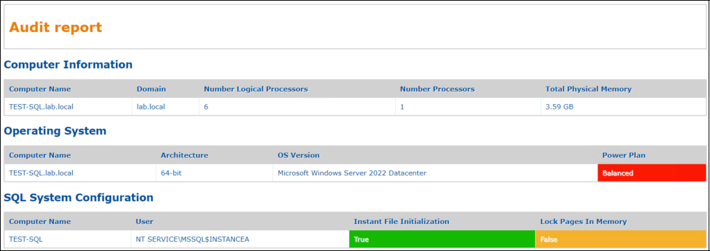 Nice to have
Let’s say I would like to add new checks. How would I proceed ?
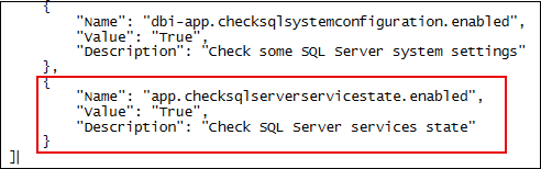
- Edit the dbi-audit-checks.ps1
- Retrieve the information related to your check
$EnableCheckSQLServerServiceState = ($AuditConfig | Where-Object { $_.Name -eq 'app.checksqlserverservicestate.enabled' } | Select-Object Value).Value- Add another function
function CheckSQLServerServiceState()
{
    if ($EnableCheckSQLServerServiceState -eq $True)
    {
        $SQLServerServiceStateList = @()
        $SQLServerServiceStateList += $Computers | Foreach-Object {
                                            Get-DbaService -ComputerName $_.Value |
                                                Select-Object ComputerName, ServiceName, ServiceType, DisplayName, StartName, State, StartMode
        }
    }

    return $SQLServerServiceStateList
}- Call it in the dbi-audit-run script
$FunctionsName = @("CheckComputersInformation", "CheckOperatingSystem", "CheckSQLSystemConfiguration", "CheckSQLServerServiceState")

$FunctionsStore = [ordered] @{}
$FunctionsStore['ComputersInformation'] = CheckComputersInformation
$FunctionsStore['OperatingSystem'] = CheckOperatingSystem
$FunctionsStore['SQLSystemConfiguration'] = CheckSQLSystemConfiguration
$FunctionsStore['SQLServerServiceState'] = CheckSQLServerServiceState
Edit the dbi-audit-stylesheet.xsl to include how you would like to display the information you collected (it’s the most consuming time part because it’s not automated. I did not find a way to automate it yet)
<body>
		    <table>
			    <tr>
				    <td>
                        <h1>Audit report</h1>
                    </td>
			    </tr>
            </table>
            <caption>
                <xsl:apply-templates select="CheckComputersInformation"/>
                <xsl:apply-templates select="CheckOperatingSystem"/>
                <xsl:apply-templates select="CheckSQLSystemConfiguration"/>
                <xsl:apply-templates select="CheckSQLServerServiceState"/>
            </caption>
        </body>

...

 <xsl:template match="CheckSQLServerServiceState">
        <h2>SQL Server Services State</h2>
	    <table>
			<tr>
				<th>Computer Name</th>
				<th>Service Name</th>
				<th>Service Type</th>
                <th>Display Name</th>
                <th>Start Name</th>
                <th>State</th>
                <th>Start Mode</th>
			</tr>
		    <tbody>
			    <xsl:apply-templates select="SQLServerServiceState"/>
		    </tbody>
	    </table>
    </xsl:template>
    <xsl:template match="SQLServerServiceState">
        <tr>
            <td><xsl:value-of select="@ComputerName"/></td>
            <td><xsl:value-of select="@ServiceName"/></td>
            <td><xsl:value-of select="@ServiceType"/></td>
            <td><xsl:value-of select="@DisplayName"/></td>
            <td><xsl:value-of select="@StartName"/></td>
            <xsl:choose>
                <xsl:when test="(@State = 'Stopped') and (@ServiceType = 'Engine')">
                    <td class="check_failed"><xsl:value-of select="@State"/></td>
                </xsl:when>
                <xsl:when test="(@State = 'Stopped') and (@ServiceType = 'Agent')">
                    <td class="check_failed"><xsl:value-of select="@State"/></td>
                </xsl:when>
                <xsl:otherwise>
                    <td class="check_passed"><xsl:value-of select="@State"/></td>
                </xsl:otherwise>
            </xsl:choose>
            <td><xsl:value-of select="@StartMode"/></td>
        </tr>
    </xsl:template>
End result :
What about sending the report through email ?
- We could add a function that send an email with an attachment.
- Edit the dbi-audit-checks file
- Add a function Send-EmailWithAuditReport
- Add this piece of code to the function :
- Edit the dbi-audit-checks file
Send-MailMessage -SmtpServer mysmtpserver -From 'Sender' -To 'Recipient' -Subject 'Audit report' -Body 'Audit report' -Port 25 -Attachments $Attachments- Edit the dbi-audit-run.ps1
- Add a call to the Send-EmailWithAuditReport function :
Send-EmailWithAuditReport -Attachments $Attachments
- Add a call to the Send-EmailWithAuditReport function :
$ReportHTMLFileName = [string]::Format("{0}\{1}_DbiAuditReport.html", $FileSavePath, (Get-Date).tostring("MM-dd-yyyy_HH-mm-ss"))

...

SendEmailsWithReport -Attachments $ReportHTMLFileName
The main idea of this solution is to be able to use the same functions while applying a different rendering. To achieve this, you would need to change the XSL stylesheet or create another XSL stylesheet and then provide to the dbi-audit-run.ps1 file the stylesheet to apply.
This would allow having the same code to perform the following tasks:
- Audit
- Health check
- …
L’article Build SQL Server audit reports with Powershell est apparu en premier sur dbi Blog.
Rancher RKE2: Rancher roles for cluster autoscaler
The cluster autoscaler brings horizontal scaling into your cluster by deploying it into the cluster to autoscale. This is described in the following blog article https://www.dbi-services.com/blog/rancher-autoscaler-enable-rke2-node-autoscaling/. It didn’t emphasize much about the user and role configuration.
With Rancher, the cluster autoscaler uses a user’s API key. We will see how to configure minimal permissions by creating Rancher roles for cluster autoscaler.
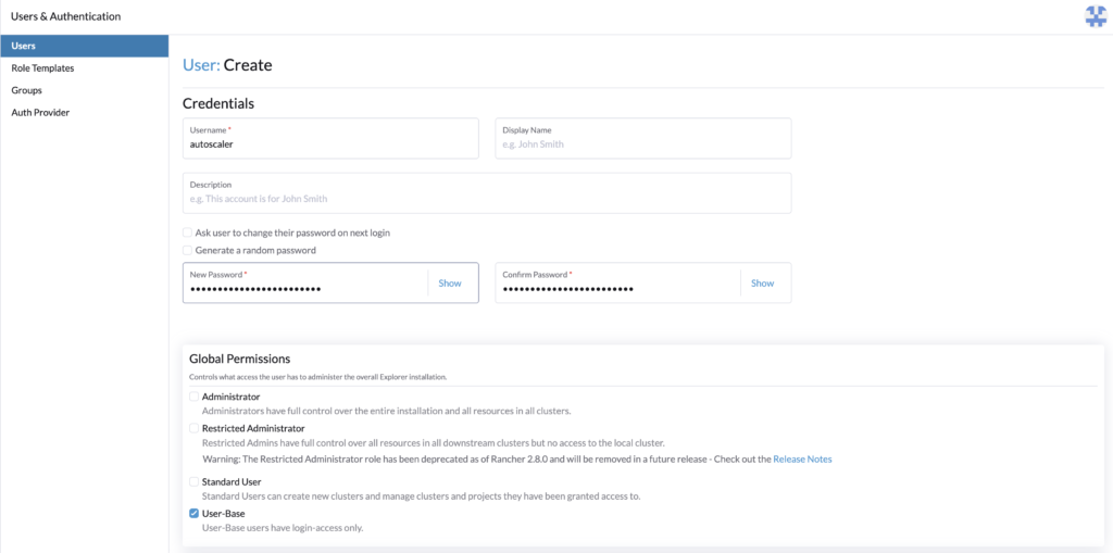
Rancher userFirst, let’s create the user that will communicate with Rancher, and whose token will be used. It will be given minimal access rights which is login access.
Go to Rancher > Users & Authentication > Users > Create.
- Set a username, for example, autoscaler
- Set the password
- Give User-Base permissions
- Create
The user is now created, let’s set Rancher roles with minimal permission for the cluster autoscaler.
Rancher roles authorizationTo make the cluster autoscaler work, the user whose API key is provided needs the following roles:
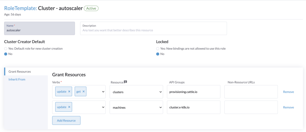
- Cluster role (for the cluster to autoscale)
Get/Update for clusters.provisioning.cattle.io
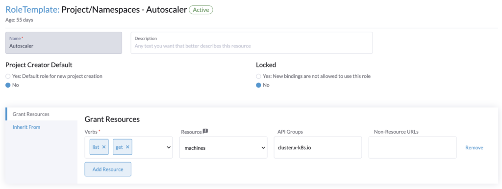
Update of machines.cluster.x-k8s.io - Project role (for the namespace that contains the cluster resource (fleet-default))
Get/List of machines.cluster.x-k8s.io
Go to Rancher > Users & Authentication > Role Templates > Cluster > Create.
Create the cluster role. This role will be applied to every cluster that we want to autoscale.
Then in Rancher > Users & Authentication > Role Templates > Project/Namespaces > Create.
Create the project role, it will be applied to the project of our local cluster (Rancher) that contains the namespace fleet-default.
 Rancher roles assignment
The user and Rancher roles are created, let’s assign them.
Project roleFirst, we will set the project role, this is to be done once.
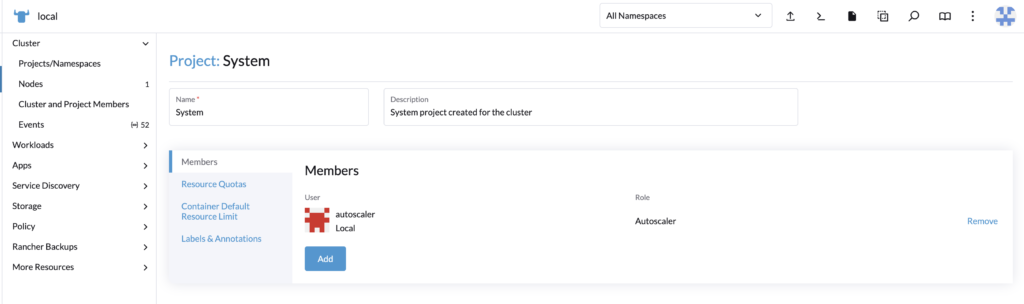
Go to the local cluster (Rancher), in Cluster > Project/Namespace.
Search for the fleet-default namespace, by default it is contained in the project System.
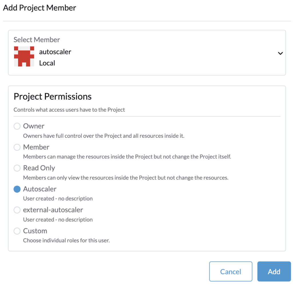
Edit the project System and add the user with the project permissions created precedently.
 Cluster role
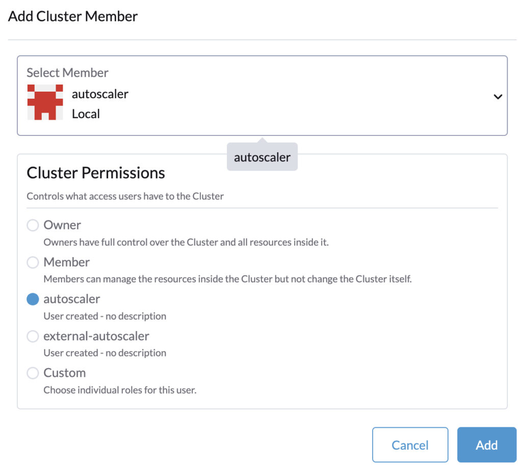
For each cluster where you will deploy the cluster autoscaler, you need to assign the user as a member with the cluster role.
In Rancher > Cluster Management, edit the cluster’s configuration and assign the user.
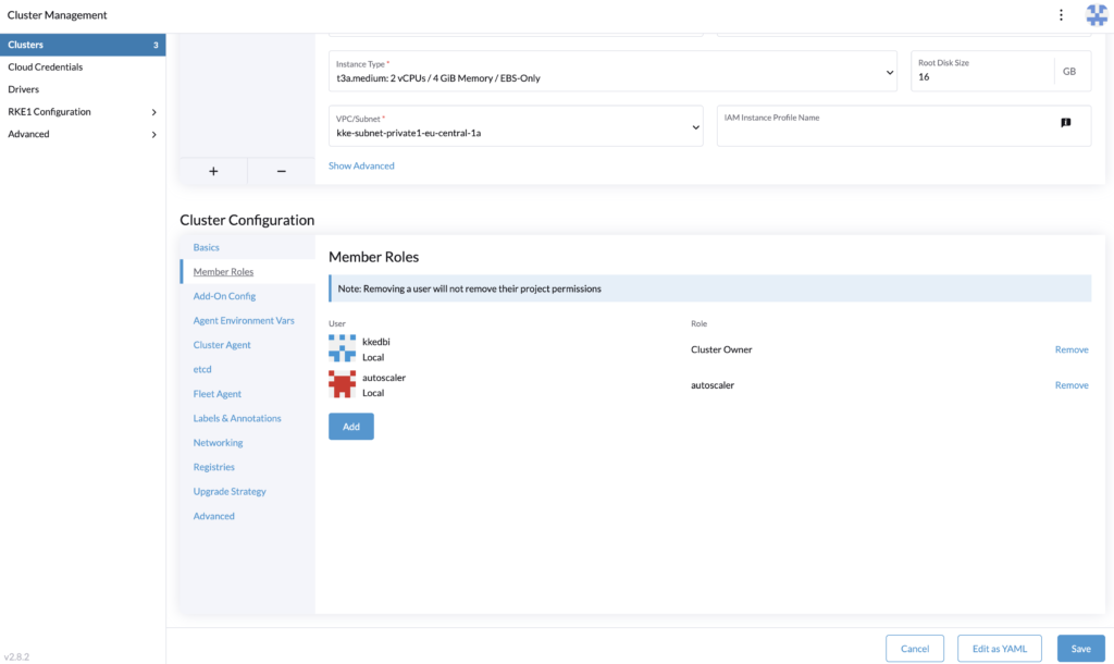
The roles assignment is done, let’s proceed to generate the token that is provided to the cluster autoscaler configuration.
Rancher API keysLog in with the autoscaler user, and go to its profile > Account & API Keys.
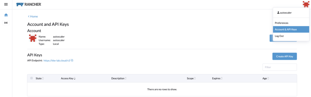
Let’s create an API Key for the cluster autoscaler configuration. Note that in a recent update of Rancher, the API keys expired by default in 90 days.
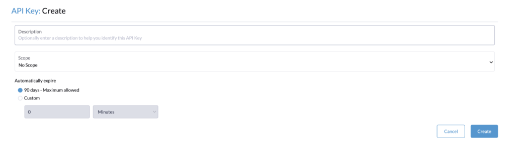
If you see this limitation, you can do the following steps to have no expiration.
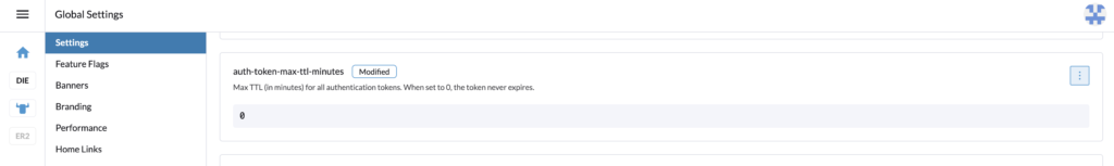
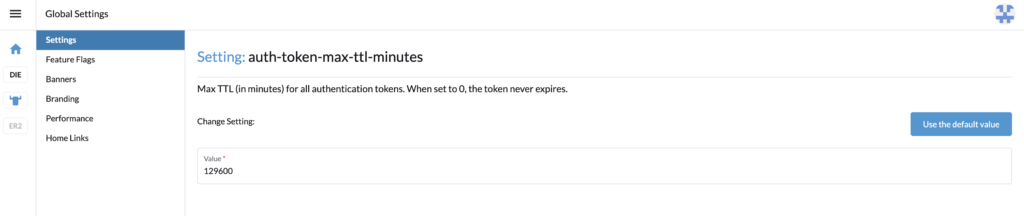
With the admin account, in Global settings > Settings, search for the setting auth-token-max-ttl-minutes and set it to 0.
Go back with the autoscaler user and create the API Key, name it for example, autoscaler, and select “no scope”.
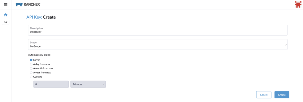
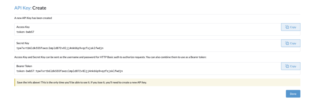
You can copy the Bearer Token, and use it for the cluster autoscaler configuration.
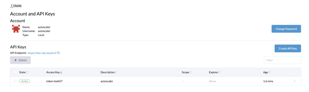
As seen above, the token never expires.
Let’s reset the parameter auth-token-max-ttl-minutes and use the default value button or the precedent value set.
We are now done with the roles configuration.
ConclusionThis blog article covers only a part of the setup for the cluster autoscaler for RKE2 provisioning. It explained the configuration of a Rancher user and Rancher’s roles with minimal permissions to enable the cluster autoscaler. It was made to complete this blog article https://www.dbi-services.com/blog/rancher-autoscaler-enable-rke2-node-autoscaling/ which covers the whole setup and deployment of the cluster autoscaler. Therefore if you are still wondering how to deploy and make the cluster autoscaler work, check the other blog.
LinksRancher official documentation: Rancher
RKE2 official documentation: RKE2
GitHub cluster autoscaler: https://github.com/kubernetes/autoscaler/tree/master/cluster-autoscaler
Blog – Rancher autoscaler – Enable RKE2 node autoscaling
https://www.dbi-services.com/blog/rancher-autoscaler-enable-rke2-node-autoscaling
Blog – Reestablish administrator role access to Rancher users
https://www.dbi-services.com/blog/reestablish-administrator-role-access-to-rancher-users/
Blog – Introduction and RKE2 cluster template for AWS EC2
https://www.dbi-services.com/blog/rancher-rke2-cluster-templates-for-aws-ec2
Blog – Rancher RKE2 templates – Assign members to clusters
https://www.dbi-services.com/blog/rancher-rke2-templates-assign-members-to-clusters
L’article Rancher RKE2: Rancher roles for cluster autoscaler est apparu en premier sur dbi Blog.
to_char a big number insert into database become scientific notation
Explain plan estimate vs actual
Elasticsearch, Ingest Pipeline and Machine Learning
Elasticsearch has few interesting features around Machine Learning. While I was looking for data to import into Elasticsearch, I found interesting data sets from Airbnb especially reviews. I noticed that it does not contain any rate, but only comments.
To have sentiment of the a review, I would rather have an opinion on that review like:
- Negative
- Positive
- Neutral
For that matter, I found the cardiffnlp/twitter-roberta-base-sentiment-latest to suite my needs for my tests.
Import ModelElasticsearch provides the tool to import models from Hugging face into Elasticsearch itself: eland.
It is possible to install it or even use the pre-built docker image:
docker run -it --rm --network host docker.elastic.co/eland/eland
Let’s import the model:
eland_import_hub_model -u elastic -p 'password!' --hub-model-id cardiffnlp/twitter-roberta-base-sentiment-latest --task-type classification --url https://127.0.0.1:9200
After a minute, import completes:
2024-04-16 08:12:46,825 INFO : Model successfully imported with id 'cardiffnlp__twitter-roberta-base-sentiment-latest'
I can also check that it was imported successfully with the following API call:
GET _ml/trained_models/cardiffnlp__twitter-roberta-base-sentiment-latest
And result (extract):
{
  "count": 1,
  "trained_model_configs": [
    {
      "model_id": "cardiffnlp__twitter-roberta-base-sentiment-latest",
      "model_type": "pytorch",
      "created_by": "api_user",
      "version": "12.0.0",
      "create_time": 1713255117150,
...
      "description": "Model cardiffnlp/twitter-roberta-base-sentiment-latest for task type 'text_classification'",
      "tags": [],
...
          },
          "classification_labels": [
            "negative",
            "neutral",
            "positive"
          ],
...
  ]
}
Next, model must be started:
POST _ml/trained_models/cardiffnlp__twitter-roberta-base-sentiment-latest/deployment/_start
This is subject to licensing. You might face this error “current license is non-compliant for [ml]“. For my tests, I used a trial.
I will use Filebeat to read review.csv file and ingest it into Elasticsearch. filebeat.yml looks like this:
filebeat.inputs:
- type: log
  paths:
    - 'C:\csv_inject\*.csv'

output.elasticsearch:
  hosts: ["https://localhost:9200"]
  protocol: "https"
  username: "elastic"
  password: "password!"
  ssl:
    ca_trusted_fingerprint: fakefp4076a4cf5c1111ac586bafa385exxxxfde0dfe3cd7771ed

  indices:
    - index: "csv"
  pipeline: csv
So each time a new file gets into csv_inject folder, Filebeat will parse it and send it to my Elasticsearch setup within csv index.
PipelineIngest pipeline can perform basic transformation to incoming data before being indexed.
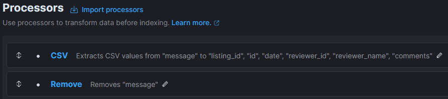
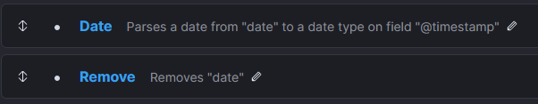
Data transformationFirst step consists of converting message field, which contains one line of data, into several target fields (ie. split csv). Next, remove message field. This looks like this in Processors section of the Ingest pipeline:
Next, I also want to replace the content of the default timestamp field (ie. @timestamp) with the timestamp of the review (and remove the date field after that):
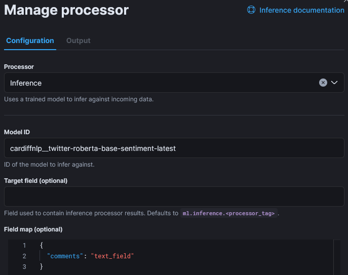
 Inference
Now, I add the Inference step:

The only customization of that step is the field map as the default input field name is “text_field“, In the reviews, fields is named “comment“:
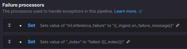
Optionally, but recommended, it is possible to add Failure processors which will set a field to keep track of the cause and will put them in a different index:
 Ingest
Now, I can simply copy the review.csv into the watched directory and Filebeat will send lines to Elasticsearch. After few minutes, I can see the first results:

Or, a considered negative example with the associated prediction rate:
 What Next?
Of course, we could try another model to compare results.
If you did not noticed, this was also a first step into Extract-transform-load topic (ETL).
L’article Elasticsearch, Ingest Pipeline and Machine Learning est apparu en premier sur dbi Blog.
Learning Azure by having fun with ChatGPT
Are you studying for an Azure certification? You may feel at some point you need a break from the dry and factual technical information. I’m in your shoes right now and I have done some experiments with ChatGPT. I’m not using it to write my text but to learn by having fun! It is very good at telling stories so why not use that for what interests me right now? Azure architecture!
In this blog post I’m going to show you how I use it, it may give you some ideas to make your learning a little more spicy!
 Prompt for preparing ChatGPT with Azure
First you’ll need to prepare ChatGPT by explaining what you want. Set the framework and limit its responses otherwise it is too chatty. As I like science fiction (sci-fi), I’m interested in a futuristic story but you could choose any style you like. My first prompt and ChatGPT response is shown below:
Act as an Azure architect. You are in charge of educating me, your student, to become an Azure architect too. You will respond to my questions by using story telling to explain each concepts requested.
I want you to:
– Always tell a simple and futuristic story
– Limit the reply to 100 words
As an Azure architect, imagine Azure as a vast cosmic city. Each service is a towering skyscraper, and we, architects, design the blueprints. Let’s start with Virtual Networks. They’re like the city’s infrastructure, connecting buildings. Subnets divide areas within each building, like floors. Next, VMs are the inhabitants, residing in these skyscrapers, each serving a unique purpose. Azure Storage, a network of secure vaults, safeguards their belongings. With Azure Load Balancer as traffic controllers, the city thrives, ensuring smooth navigation. As architects of this digital metropolis, we sculpt a future where innovation soars amidst the azure skyline.
Not bad! It gives me some key components of an Azure infrastructure and makes some analogies I can easily picture in my head. With this basis, I can now be the hero of this story by asking more questions.
Build up that Azure cosmic city with ChatGPTYou can then ask questions around your area of study (mine is Azure architecture) and stay immersed into that story. For example:
What are the best practice to govern this Azure cosmic city?
In our cosmic city, governance is paramount. Azure Policy acts as the city’s constitution, ensuring compliance with regulations. Role-Based Access Control (RBAC) assigns roles to citizens, granting appropriate permissions. Azure Resource Manager templates are like city blueprints, ensuring consistency in construction. Tags label buildings for easy identification, while Azure Monitor keeps a watchful eye on city activities. With these best practices, our cosmic city thrives, ensuring order, security, and harmony amidst the azure skyline.It gives you the key elements of Azure governance by continuing its story. You can go on like this back and forth by throwing in any chapter of your course. You can focus on a specific use case as well and see how it integrates with this story:
How can I migrate my SQL Server database on-premises to this city?
Imagine your SQL Server database as a cozy cottage in the countryside. To migrate to our cosmic city, Azure, we’ll use Azure Database Migration Service, like a futuristic moving company. It carefully transports your data to Azure SQL Database, a sleek skyscraper in our city. With minimal downtime, your database seamlessly transitions to its new home, ready to thrive amidst the azure skyline. Just sit back, relax, and watch as your data becomes part of the bustling digital metropolis.How do I ensure my database is highly resilient in this cosmic city?
In our cosmic city, resilience is key. Azure offers a robust solution: Azure SQL Database with built-in redundancy, akin to a fortress with multiple layers of defense. Automatic backups act as a safety net, ensuring data is never lost. Geo-replication creates duplicates across regions, safeguarding against disasters. With Azure SQL Database’s high availability and disaster recovery features, your database thrives amidst the azure skyline, resilient against any digital storm.I don’t know if it works for you but I find it fascinating I can make ChatGPT talk endlessly and respond to any questions I have about Azure in a sci-fi story!
Dive into an Azure componentAs usual with ChatGPT you need to drive the discussion to get the most of it. Let’s see what it has to say about Azure AD (I use the legacy terminology as ChatGPT v3.5 doesn’t know yet Microsoft Entra ID):
What and where would be the Azure AD in this city?
In our bustling city, Azure AD is the central hub, akin to City Hall. It’s where identities are registered, like citizens in our digital society. Located at the heart of the city, Azure AD ensures secure access to every digital service and resource, much like City Hall grants access to essential services. From authentication to authorization, Azure AD governs the city’s digital identities, ensuring a seamless and secure experience for all inhabitants amidst the azure skyline.How would Azure AD conditional access be implemented in this city?
In our city, Azure AD Conditional Access acts as the city’s security checkpoints. Picture futuristic gates at key entry points, only granting access to authorized individuals based on specific conditions. Want to enter the financial district skyscraper? You’ll need more than just a pass; perhaps a biometric scan during business hours. Conditional Access ensures only the right people, with the right permissions, access sensitive areas of our digital city. It’s our shield against cyber threats amidst the azure skyline, ensuring a safe and secure digital environment for all inhabitants.How would I connect from my Active Directory in the countryside to this Azure AD in the cloud?
In the countryside, your Active Directory (AD) is like a quaint village square, bustling with local identities. To connect to Azure AD in our cosmic cloud city, envision a digital bridge spanning the distance between village and skyline. Azure AD Connect is your trusty guide, seamlessly synchronizing identities from countryside AD to Azure AD. With this bridge in place, villagers can access digital services in the cloud using their familiar countryside credentials. Just like that, the countryside becomes an integral part of our digital metropolis, united under the azure skyline.You can then piece by piece for each component create a complete city in the countryside (OnPrem) and in the cloud and illustrate their interaction. We could completely gamify this! SimCity anyone?
LimitationsSome general concepts are more difficult to put into a visual story as for example the Microsoft Cloud Adoption Framework:
What would be the Microsoft Cloud Adoption Framework for Azure in this city?
In our dynamic metropolis, the Microsoft Cloud Adoption Framework for Azure is our roadmap to success. Like a futuristic GPS, it guides us through the twists and turns of digital transformation. Envisioning helps us set our destination, planning ensures we choose the best route, and readiness prepares us for the journey ahead. Migration helps us seamlessly transition, while innovation propels us forward. With governance as our compass and optimization as our fuel, we navigate the ever-changing landscape, building a future where our digital city thrives amidst the azure skyline. Ready to embark on this transformative journey?I don’t find it fantastic as we recognize the empty blabbering of ChatGPT. We would need to be more specific to get something more interesting.
Wrap upYou can see how by relaxing from your studies, you can still continue to learn by having fun in an imaginary world. You could totally convert all this into visual notes that will help you when you renew your certifications. That is something I’m starting to explore.
This is just a glimpse of how you could use ChatGPT in your journey to learn Azure or anything else. Brainstorm any concept, service or component you are learning and see how it integrates into a visual story to get a high-level picture. Let me know if your are using ChatGPT that way for learning and what is the world you are building for it!
L’article Learning Azure by having fun with ChatGPT est apparu en premier sur dbi Blog.